Squeezing out Postgres performance on RTABench Q0

Some doubtful aspects of the optimiser

I often hear that PostgreSQL is not suitable for solving analytics problems, referencing TPC-H or ClickBench results as evidence. Surely, handling a straightforward task like sorting through 100 million rows on disk and calculating a set of aggregates, you would get stuck on the storage format and parallelisation issues that limit the ability to optimise the DBMS.

In practice, queries tend to be highly selective and do not require processing extensive rows. The focus, then, shifts to the order of JOIN operations, caching intermediate results, and minimising sorting operations. In these scenarios, PostgreSQL, with its wide range of query execution strategies, can indeed have an advantage.

I wanted to explore whether Postgres could be improved by thoroughly utilising all available tools, and for this, I chose the RTABench benchmark. RTABench is a relatively recent benchmark that is described as being close to real-world scenarios and highly selective. One of its advantages is that the queries include expressions involving the JSONB type, which can be challenging to process. Additionally, the Postgres results on RTABench have not been awe-inspiring.

Ultimately, I decided to review all of the benchmark queries, and fortunately, there aren't many, to identify possible optimisations. However, already on the zero query, there were enough nuances that it was worth taking it out into a separate discussion.

My setup isn't the latest - it's a MacBook Pro from 2019 with an Intel processor—so we can't expect impressive or stable performance metrics. Instead, let's concentrate on qualitative characteristics rather than quantitative ones. For this purpose, my hardware setup should be sufficient. You can find the list of non-standard settings for the Postgres instance here.

Now, considering the zero RTABench query, which involves calculating several aggregates over a relatively small sample from the table:

EXPLAIN (ANALYZE, BUFFERS ON, TIMING ON, SETTINGS ON)
WITH hourly_stats AS (
  SELECT 
    date_trunc('hour', event_created) as hour,
    event_payload->>'terminal' AS terminal,
    count(*) AS event_count
  FROM order_events
  WHERE 
    event_created >= '2024-01-01' AND
    event_created < '2024-02-01'
    AND event_type IN ('Created', 'Departed', 'Delivered')
  GROUP BY hour, terminal
)
SELECT 
  hour,
  terminal,
  event_count,
  AVG(event_count) OVER (
    PARTITION BY terminal
    ORDER BY hour
    ROWS BETWEEN 3 PRECEDING AND CURRENT ROW
  ) AS moving_avg_events
FROM hourly_stats
WHERE terminal IN ('Berlin', 'Hamburg', 'Munich')
ORDER BY terminal, hour;

Phase 0. ‘Default behaviour‘

The query does not seem surprising. Let's run a query over the default data schema (EXPLAIN has been cleaned):

WindowAgg  (actual time=21053.119 rows=2232)
  Window: w1 AS (PARTITION BY
   order_events.event_payload ->> 'terminal'
   ORDER BY date_trunc('hour', order_events.event_created))
  Buffers: shared read=3182778
  -> Sort  (actual time=21052.476 rows=2232)
     Sort Key:
      order_events.event_payload ->> 'terminal',
      date_trunc('hour', order_events.event_created)
      Sort Method: quicksort  Memory: 184kB
   -> GroupAggregate  (actual time=21051.875 rows=2232)
       Group Key:
        date_trunc('hour', order_events.event_created),
        order_events.event_payload ->> 'terminal'
     -> Sort (actual time=21037.609..21042.766 rows=204053)
         Sort Key:
          date_trunc('hour', order_events.event_created),
          order_events.event_payload ->> 'terminal'
         Sort Method: quicksort  Memory: 12521kB
       -> Bitmap Heap Scan on order_events
            (actual time=20999.978 rows=204053)
          Recheck Cond: event_type =
           ANY ('{Created,Departed,Delivered}')
          Filter:
           event_created >= '2024-01-01 00:00:00+00' AND
           event_created < '2024-02-01 00:00:00+00' AND
           event_payload ->> 'terminal') =
             ANY ('{Berlin,Hamburg,Munich}')
          Rows Removed by Filter: 57210049
          Heap Blocks: exact=3133832
          Buffers: shared read=3182778
        -> Bitmap Index Scan (actual time=1683.357 rows=57414102)
           Index Cond: event_type = ANY ('{Created,Departed,Delivered}')
           Index Searches: 1
           Buffers: shared read=48946
Execution Time: 21060.564 ms

The execution time is 21 seconds? Really? Seems too slow. Upon examining the EXPLAIN, we realise that the main issue is that the default schema contains only one low-selectivity index, which was used during execution instead of performing a sequential scan. The EXPLAIN also indicates that a significant portion of the work involves collecting identifiers (ctid) of candidate rows, which takes 1.6 seconds. Following that, filtering through these rows results in filtering out 98% of the read rows, which takes 19 seconds.

The first problem was identified quickly: I allocated 8GB for shared_buffers; however, the DBMS limits the amount of buffer space that can be assigned to a single table. The formula for this allocation is quite complex, involving multiple factors, but the NBuffers/MaxBackends ratio applies here. Consequently, with my current settings, PostgreSQL can allocate a maximum of only 2.4GB per table. Therefore, denormalising the entire database into one wide, long table is a bad idea in PostgreSQL, at least for this reason.

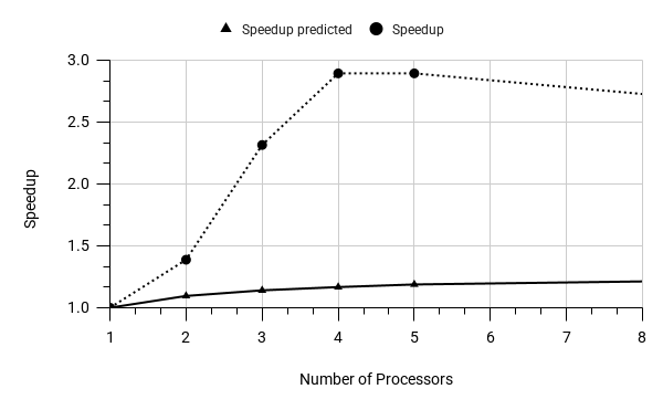
Despite the data access pattern in this query plan being somewhat inefficient, let’s first try a straightforward approach to improve the performance by increasing the number of parallel workers:

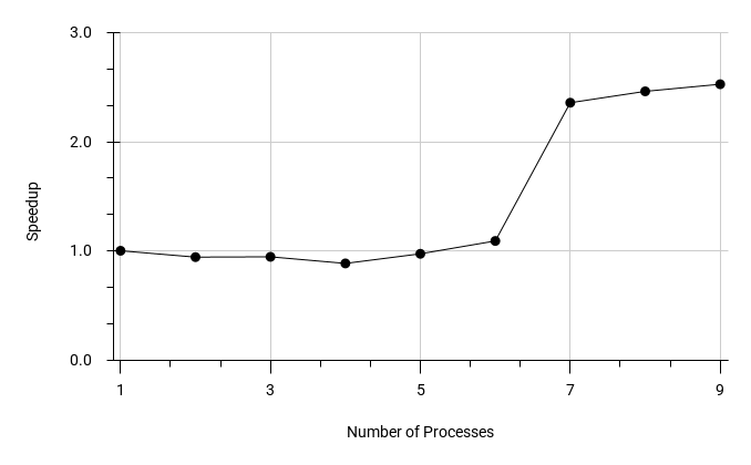
A very strange graph. Obviously, suppose most of the work is reading from disk and the tuple deformation. In that case, one should not expect a significant effect from parallelism. But where does this jump between 6 and 7 parallel processes come from? Looking at the EXPLAINs, one can easily understand - there was a change in the query plan. BitmapScan was used on a small number of workers, and the optimiser picked SeqScan on a larger number.

So maybe SeqScan should have been used on a small number of workers, too? Let's see how the scanning operation is accelerated separately for BitmapScan and SeqScan, and also watch how the costs of the scanning nodes change (in relative values):

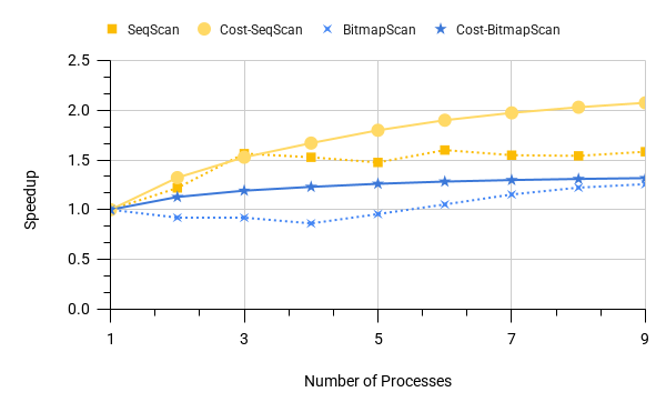
Raw numbers and EXPLAINs can be found here and here.

The thing is that for a small number of workers, BitmapScan has a smaller cost than SeqScan, which in our case does not correlate with execution time. The point here is probably in a delicate balance: 'fewer lines read / but more often went from the index to the table'. It is difficult to say more precisely, since explain does not show such details of the estimate as the expected number of tuples fetched from the disk before filtering, an estimate of the number of fetched disk pages, or an estimate of the proportion of pages that will be found in shared_buffers. On the other hand, the cost model assumes better scalability of SeqScan compared to BitmapScan, which causes the plan to switch to SeqScan. Considering that for SeqScan, a change in the cost value predicts an unreasonably significant increase in performance, this may result in selecting a SeqScan method where it should not. Thus, for now, you should be careful optimising queries by increasing the number of parallel workers.

Phase 1. ‘Typical optimisation‘

Now let's move on and see what a good index will give Postgres. A typical practice is to create an index on the most frequently used highly selective column in filters. For this query, the choice is limited to only one option:

CREATE INDEX idx_1 ON order_events (event_created);

With this index, the optimiser utilises IndexScan to access data, reducing the query execution time (without parallel workers) to 6.5 seconds. Interestingly, the previous query plan accessed buffer pages 3 million times (shared read = 3182778), while in this case, with a more selective scan, it increased to 14 million (shared hit = 14317527). Although there are more trips to the buffer now, in the previous example, each page replaced a previous one in the buffer. In contrast, both the index and the disk pages now fit into the shared buffers, which contributes to the acceleration.

Next, let's explore whether parallel workers will provide additional benefits and examine how the cost model predicts this outcome:

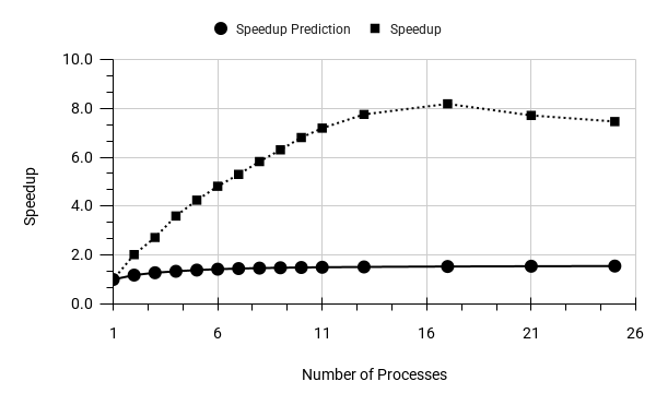
Raw data can be taken here.

Yes, we see some acceleration. The parallelisation effect goes so far that we have to expand the permissible number of workers to 24 to track the impact to the end. And here one of the disadvantages of Postgres showed itself. Although we set all possible hooks to large values, the optimiser hit a hard-wired limit on the number of workers (10 for this table) on the order_events table. We had to bypass it with the command:

ALTER TABLE order_events SET (parallel_workers = 32);

It is pretty sad that the number of workers implicitly depends on the table size estimate. This can be a problem, for example, in the JOIN operator, which determines the required number of workers based on the number of workers requested on the outer side of the join. It is easy to imagine a situation where a petite table, insufficient even for one parallel worker, and a very large one are joined. In this case, the entire jointree may remain non-parallelised just because of one small table!

Another fact can be extracted from the above graph - the cost model for Index Scan is very conservative: with the maximum observed speedup of 8, the model did not show even a two-fold speedup. Hence the conclusions: 1) when using indexes, do not be shy about raising worker limits, and 2) Scan nodes that are more sensitive to the number of workers (we observed this, for example, with SeqScan), can unexpectedly trigger a rebuild of the query plan for the worse.

However, the current index is not the ultimate dream. Let's take a closer look at the scanning node:

Index Scan (actual time=6555.122 rows=204053)
  Index Cond: event_created >= '2024-01-01 00:00:00+00' AND
    event_created < '2024-02-01 00:00:00+00'
  Filter: event_type = ANY ('{Created,Departed,Delivered}' AND
    event_payload ->> 'terminal' = ANY ('{Berlin,Hamburg,Munich}')
  Rows Removed by Filter: 14099758
  Index Searches: 1
  Buffers: shared hit=14317527

Lots of pages touched, lots of lines filtered. Let's see what can be achieved by minimising disk reads.

Phase 2. ‘Reinforced optimisation‘

In this section, we will confidently assume the existence of an 'index adviser' that helps analyse and automatically create composite indexes. These indexes optimise data retrieval by minimising the reading of table rows, thereby adapting the entire system to the incoming load.

In this query, we have several options to consider. We will exclude the GIN index because the event_payload column lacks selectivity. This leaves us with two alternative options:

CREATE INDEX idx_2 ON order_events (event_created, event_type)
  INCLUDE (event_payload);
CREATE INDEX idx_3 ON order_events (event_created, event_type);

The idx_2 variant does not require accessing the table at all, while the idx_3 index can cause both IndexScan and BitmapScan. You can find various EXPLAINs of these indexes here. It’s interesting to note that with the previously created idx_1 index, adding idx_2 does not result in switching to the obviously faster IndexOnlyScan. This suggests that when evaluating the cost of index access, the width of the index plays a significant role. The jsonb field likely increases the size of idx_2 considerably.

Consequently, the idx_3 index has proven to be the most optimal in terms of compactness and the number of selected records when using the BitmapScan method. By closely examining the scanning nodes, we can understand the reasons behind this conclusion:

Bitmap Heap Scan (actual time=1286.430 rows=204053
  Rows Removed by Filter: 4292642
  Heap Blocks: exact=269237
  Buffers: shared hit=313925
  Bitmap Index Scan (actual time=625.170 rows=4496695)
    Index Searches: 1
    Buffers: shared hit=44688

Index Only Scan (actual time=1586.097 rows=204053)
  Rows Removed by Filter: 4292642
  Heap Fetches: 0
  Index Searches: 1
  Buffers: shared hit=2558314

Index Scan (actual time=2847.517 rows=204053)
  Rows Removed by Filter: 4292642
  Index Searches: 1
  Buffers: shared hit=4509185

All three index scans return the same number of rows, perform a single pass through the index, and filter the same number of rows. However, IndexOnlyScan wins over Index Scan due to the fact that it does not go into the table and touches the buffer pages twice as rarely (2.6 million V/S 4.5 million); BitmapScan goes into the buffer even less often (300 thousand times) - after going through the index and collecting tid of candidate rows, it then goes pointwise to the heap, touching each potentially useful page only once.

Let's see how parallel workers now help speed up the query for each type of scanning:

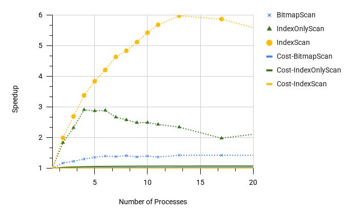
It turns out that in the case of BitmapScan, there is no particular sense in using workers. Having a significant computing resource and low competition between clients, it is worth considering reducing the cost (see the parallel_setup_cost and parallel_tuple_cost parameters) of parallel execution and disabling BitmapScan.

However, the cost model again turned out to be insensitive to the effect of parallelism. And first of all, something should be done here. It was also noted that with 8+ workers, the plan was again rebuilt on SeqScan, which led to an increase in execution time from ~1c to ~21c. Therefore, in the interests of the experiment, SeqScan had to be manually disabled.

However, even with such a good index, we see that a certain number of lines have to be filtered. Let's go all the way and organise selective access to only relevant data.

Phase 3. ‘Crazy optimisation‘

Let's now try to reach the theoretical limit of optimisation of this query. Here, we can imagine having an advanced 'Disk Access Tuner' that analyses various expressions of the SQL query to find combinations of high and low selective filters on the same table, which is a good reason to consider partial indexes. Let's create the following ideal index:

CREATE INDEX idx_5 ON order_events (event_created, event_type)
INCLUDE (event_payload)
WHERE
  event_created >= '2024-01-01' and event_created < '2024-02-01' AND
  event_type IN ('Created', 'Departed', 'Delivered') AND
  (event_payload ->> 'terminal') = ANY ('{Berlin,Hamburg,Munich}');

The index is designed so that no table access is necessary, and all rows in this index are relevant to the query. Therefore, there is no need to evaluate the filter value, which also helps save CPU time during the execution. The base case (without workers) now executes in 54 ms (as shown in the EXPLAINs here).

In such a straightforward scenario, it's clear that the estimation of the cardinality for the scan operator is made with an error:

Index Only Scan (cost=0.42..4998.13 rows=70210)
                (actual time=34.718 rows=204053.00 loops=1)
    Heap Fetches: 0
    Index Searches: 1
    Buffers: shared hit=110862

Scanning does not rely on a filter; the table is, in fact, static, yet it still makes errors! In this instance, it may not be significant, but if there were a join tree above, an incorrect estimate at a leaf node could lead to a substantial error when selecting a join strategy. Why can't the optimiser refine the selectivity of the sample based on the existing indexes? Let's also explore whether scaling is effective here with parallel workers. Due to the increased share of the remaining (non-parallel) portion of the query, we will focus solely on the actual time and estimated cost of the scan nodes themselves:

Here, as in the previous case, it is clear that the IndexOnlyScan scanning effect ends at three workers. But the cost model does not even show this. Why does the cost model reflect the real numbers so poorly? Perhaps it is conservative due to the diversity of hardware parallelism models and, as a result, the different impact of parallelisation on the query execution. Or maybe there is an implicit assumption that there is a neighbouring backend nearby that will compete for the resource? In any case, I would personally like to have an explicit parameter that allows me to configure this effect, given the nature of my system's load.

Conclusion

What lessons can be drawn from this simple experiment?

1. Parallel workers significantly affect performance, so it's vital to adjust the optimiser's cost model to align with the server's capabilities, increasing the proportion of parallel plans and the number of workers.

2. The efficiency of parallelisation is highly dependent on the access technique, and preference should be given to IndexScan over BitmapScan, SeqScan and even IndexOnlyScan.

3. It appears that the cost model for parallelism in PostgreSQL has not been sufficiently polished, potentially leading to side effects such as defaulting to inefficient SeqScan operations.

4. Considering the weak points of the current PostgreSQL row storage, it lacks the ability to adjust the set of indexes to optimise data access based on the actual workload.

5. More deeply employing indexes in the planning process may provide worthwhile improvements in cardinality estimations.

THE END.
July 26, 2025, Madrid, Spain.